علم الكيمياء

تاريخ الكيمياء والعلماء المشاهير
التحاضير والتجارب الكيميائية
المخاطر والوقاية في الكيمياء
اخرى
مقالات متنوعة في علم الكيمياء
كيمياء عامة
الكيمياء التحليلية
مواضيع عامة في الكيمياء التحليلية
التحليل النوعي والكمي
التحليل الآلي (الطيفي)
طرق الفصل والتنقية
الكيمياء الحياتية
مواضيع عامة في الكيمياء الحياتية
الكاربوهيدرات
الاحماض الامينية والبروتينات
الانزيمات
الدهون
الاحماض النووية
الفيتامينات والمرافقات الانزيمية
الهرمونات
الكيمياء العضوية
مواضيع عامة في الكيمياء العضوية
الهايدروكاربونات
المركبات الوسطية وميكانيكيات التفاعلات العضوية
التشخيص العضوي
تجارب وتفاعلات في الكيمياء العضوية
الكيمياء الفيزيائية
مواضيع عامة في الكيمياء الفيزيائية
الكيمياء الحرارية
حركية التفاعلات الكيميائية
الكيمياء الكهربائية
الكيمياء اللاعضوية
مواضيع عامة في الكيمياء اللاعضوية
الجدول الدوري وخواص العناصر
نظريات التآصر الكيميائي
كيمياء العناصر الانتقالية ومركباتها المعقدة
مواضيع اخرى في الكيمياء
كيمياء النانو
الكيمياء السريرية
الكيمياء الطبية والدوائية
كيمياء الاغذية والنواتج الطبيعية
الكيمياء الجنائية
الكيمياء الصناعية
البترو كيمياويات
الكيمياء الخضراء
كيمياء البيئة
كيمياء البوليمرات
مواضيع عامة في الكيمياء الصناعية
الكيمياء التناسقية
الكيمياء الاشعاعية والنووية

The uncertainty principle
 المؤلف:
Peter Atkins، Julio de Paula
المؤلف:
Peter Atkins، Julio de Paula
 المصدر:
ATKINS PHYSICAL CHEMISTRY
المصدر:
ATKINS PHYSICAL CHEMISTRY
 الجزء والصفحة:
ص269-272
الجزء والصفحة:
ص269-272
 2025-11-22
 317
317


+
-
20
The uncertainty principle
We have seen that, if the wavefunction is Aeikx, then the particle it describes has a definite state of linear momentum, namely travelling to the right with momentum px =+kh. However, we have also seen that the position of the particle described by this wavefunction is completely unpredictable. In other words, if the momentum is specified precisely, it is impossible to predict the location of the particle. This statement is one-half of a special case of the Heisenberg uncertainty principle, one of the most celebrated results of quantum mechanics: It is impossible to specify simultaneously, with arbitrary precision, both the momentum and the position of a particle. Before discussing the principle further, we must establish its other half: that, if we know the position of a particle exactly, then we can say nothing about its momentum. The argument draws on the idea of regarding a wavefunction as a superposition of eigenfunctions, and runs as follows. If we know that the particle is at a definite location, its wavefunction must be large there and zero everywhere else (Fig. 8.30). Such a wavefunction can be created by superimposing a large number of harmonic (sine and cosine) functions, or, equivalently, a number of eikx functions. In other words, we can create a sharply localized wavefunction, called a wave packet, by forming a linear combination of wave functions that correspond to many different linear momenta. The superposition of a few harmonic functions gives a wavefunction that spreads over a range of locations (Fig. 8.31). However, as the number of wavefunctions in the superposition increases, the wave packet becomes sharper on account of the more complete interference between the positive and negative regions of the individual waves. When an infinite number of components is used, the wave packet is a sharp, infinitely narrow spike, which corresponds to perfect localization of the particle. Now the particle is perfectly localized. However, we have lost all information about its momentum because, as we saw above, a measurement of the momentum will give a result corresponding to any one of the infinite number of waves in the superposition, and which one it will give is unpredictable. Hence, if we know the location of the particle precisely (implying that its wavefunction is a superposition of an infinite number of momentum eigen functions), then its momentum is completely unpredictable. A quantitative version of this result is , ∆p∆q≥ 1/2h , In this expression ∆p is the ‘uncertainty’ in the linear momentum parallel to the axis q, and ∆q is the uncertainty in position along that axis. These ‘uncertainties’ are precisely defined, for they are the root mean square deviations of the properties from their mean values:
∆p= {p2 − p2}1/2 ∆q={q2 − q2}1/2
If there is complete certainty about the position of the particle (∆q = 0), then the only way that eqn 8.36a can be satisfied is for ∆p =∞, which implies complete uncertainty about the momentum. Conversely, if the momentum parallel to an axis is known exactly (∆p = 0), then the position along that axis must be completely uncertain (∆q =∞).
The p and q that appear in eqn 8.36 refer to the same direction in space. Therefore, whereas simultaneous specification of the position on the x-axis and momentum parallel to the x-axis are restricted by the uncertainty relation, simultaneous location of position on x and motion parallel to y or z are not restricted. The restrictions that the uncertainty principle implies are summarized in Table 8.2.
The Heisenberg uncertainty principle is more general than eqn 8.36 suggests. It applies to any pair of observables called complementary observables, which are defined in terms of the properties of their operators. Specifically, two observables Ω1 andΩ2are complementary if
When the effect of two operators depends on their order (as this equation implies), we say that they do not commute. The different outcomes of the effect of applying)1 and)2in a different order are expressed by introducing the commutator of the two operators, which is defined as
We can conclude from Illustration 8.3 that the commutator of the operators for position and linear momentum is
The commutator in eqn 8.39 is of such vital significance in quantum mechanics that it is taken as a fundamental distinction between classical mechanics and quantum mechanics. In fact, this commutator may be taken as a postulate of quantum mechanics, and is used to justify the choice of the operators for position and linear momentum given in eqn 8.26.
With the concept of commutator established, the Heisenberg uncertainty principle can be given its most general form. For any two pairs of observables, Ω1 and Ω2, the uncertainties (to be precise, the root mean square deviations of their values from the mean) in simultaneous determinations are related by
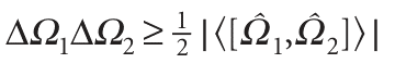
We obtain the special case of eqn 8.36a when we identify the observables with x and px and use eqn 8.39 for their commutator. Complementary observables are observables with non-commuting operators. With the discovery that some pairs of observables are complementary (we meet more examples in the next chapter), we are at the heart of the difference between classical and quantum mechanics. Classical mechanics supposed, falsely as we now know, that the position and momentum of a particle could be specified simultaneously with arbitrary precision. However, quantum mechanics shows that position and momentum are complementary, and that we have to make a choice: we can specify position at the expense of momentum, or momentum at the expense of position. The realization that some observables are complementary allows us to make considerable progress with the calculation of atomic and molecular properties, but it does away with some of the most cherished concepts of classical physics.
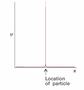
Fig. 8.30 The wavefunction for a particle at a well-defined location is a sharply spiked function that has zero amplitude everywhere except at the particle’s position.
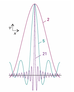
Fig. 8.31 The wavefunction for a particle with an ill-defined location can be regarded as the superposition of several wavefunctions of definite wavelength that interfere constructively in one place but destructively elsewhere. As more waves are used in the superposition (as given by the numbers attached to the curves), the location becomes more precise at the expense of uncertainty in the particle’s momentum. An infinite number of waves is needed to construct the wavefunction of a perfectly localized particle.
 الاكثر قراءة في مواضيع عامة في الكيمياء الفيزيائية
 اخر الاخبار
اخبار العتبة العباسية المقدسة

الآخبار الصحية


 قسم الشؤون الفكرية يصدر كتاباً يوثق تاريخ السدانة في العتبة العباسية المقدسة
 "المهمة".. إصدار قصصي يوثّق القصص الفائزة في مسابقة فتوى الدفاع المقدسة للقصة القصيرة
 (نوافذ).. إصدار أدبي يوثق القصص الفائزة في مسابقة الإمام العسكري (عليه السلام)