
Operators, eigenvalues, and eigenfunctions
 المؤلف:
Peter Atkins، Julio de Paula
المؤلف:
Peter Atkins، Julio de Paula
 المصدر:
ATKINS PHYSICAL CHEMISTRY
المصدر:
ATKINS PHYSICAL CHEMISTRY
 الجزء والصفحة:
ص261-264
الجزء والصفحة:
ص261-264
 2025-11-22
 18
18
Operators, eigenvalues, and eigenfunctions
To formulate a systematic way of extracting information from the wavefunction, we first note that any Schrödinger equation (such as those in eqns 8.13 and 8.18) may be written in the succinct form , Hψ=Eψ , with (in one dimension)

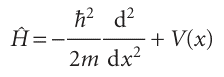
The quantity @ is an operator, something that carries out a mathematical operation on the function ψ. In this case, the operation is to take the second derivative of ψ and (after multiplication by −$2/2m) to add the result to the outcome of multiplying ψ by V. The operator @ plays a special role in quantum mechanics, and is called the hamiltonian operator after the nineteenth century mathematician William Hamilton, who developed a form of classical mechanics that, it subsequently turned out, is well suited to the formulation of quantum mechanics. The hamiltonian operator is the operator corresponding to the total energy of the system, the sum of the kinetic and potential energies. Consequently, we can infer—as we anticipated in Section 8.3— that the first term in eqn 8.24b (the term proportional to the second derivative) must be the operator for the kinetic energy. When the Schrödinger equation is written as in eqn 8.24a, it is seen to be an eigenvalue equation, an equation of the form
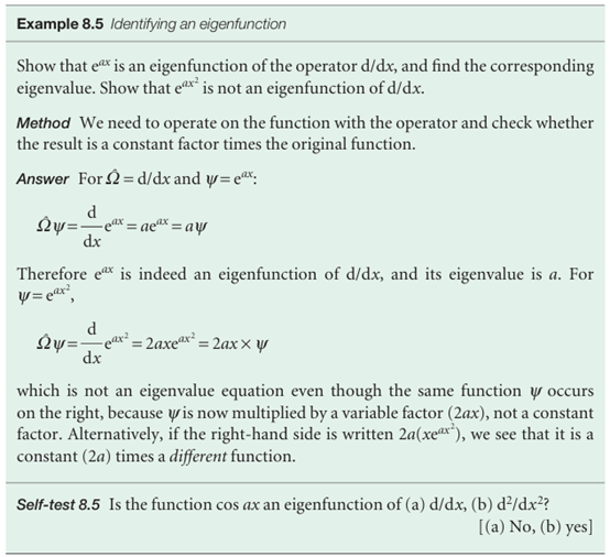
(Operator)(function) = (constant factor) × (same function) , If we denote a general operator by) (where Ω is uppercase omega) and a constant factor by ω (lowercase omega), then an eigenvalue equation has the form , Ω ψ=ωψ , The factor ω is called the eigenvalue of the operator Ω. The eigenvalue in eqn 8.24a is the energy. The function ψ in an equation of this kind is called an eigenfunction of the operator Ω and is different for each eigenvalue. The eigenfunction in eqn 8.24a is the wavefunction corresponding to the energy E. It follows that another way of saying ‘solve the Schrödinger equation’ is to say ‘find the eigenvalues and eigen functions of the hamiltonian operator for the system’. The wavefunctions are the eigenfunctions of the hamiltonian operator, and the corresponding eigenvalues are the allowed energies.
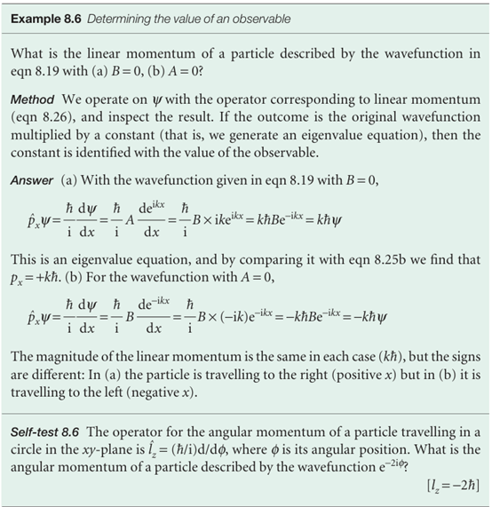
The importance of eigenvalue equations is that the pattern (Energy operator) ψ = (energy) × ψ , exemplified by the Schrödinger equation is repeated for other observables, or measur-able properties of a system, such as the momentum or the electric dipole moment. Thus, it is often the case that we can write , (Operator corresponding to an observable)ψ = (value of observable) × ψ , The symbol Ω in eqn 8.25b is then interpreted as an operator (for example, the hamiltonian, H) corresponding to an observable (for example, the energy), and the eigenvalue ω is the value of that observable (for example, the value of the energy, E). Therefore, if we know both the wavefunction ψ and the operator Ω corresponding to the observable Ω of interest, and the wavefunction is an eigenfunction of the operator Ω, then we can predict the outcome of an observation of the property Ω (for example, an atom’s energy) by picking out the factor ω in the eigenvalue equation, eqn 8.25b.
A basic postulate of quantum mechanics tells us how to set up the operator corresponding to a given observable: Observables, Ω, are represented by operators, Ω, built from the following position and momentum operators:
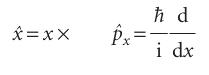
That is, the operator for location along the x-axis is multiplication (of the wavefunction) by x and the operator for linear momentum parallel to the x-axis is proportional to taking the derivative (of the wavefunction) with respect to x.
We use the definitions in eqn 8.26 to construct operators for other spatial observables. For example, suppose we wanted the operator for a potential energy of the form V= 1/2 kx2, with k a constant (later, we shall see that this potential energy describes the vibrations of atoms in molecules). Then it follows from eqn 8.26 that the operator corresponding to V is multiplication by x2:
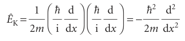
W= 1/2kx2× , In normal practice, the multiplication sign is omitted. To construct the operator for kinetic energy, we make use of the classical relation between kinetic energy and linear momentum, which in one dimension is EK=px2/2m. Then, by using the operator for px in eqn 8.26 we find:
It follows that the operator for the total energy, the hamiltonian operator, is
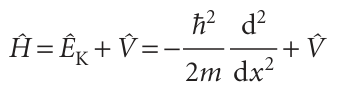
With V the multiplicative operator in eqn 8.27 (or some other relevant potential energy). The expression for the kinetic energy operator, eqn 8.28, enables us to develop the point made earlier concerning the interpretation of the Schrödinger equation. In mathematics, the second derivative of a function is a measure of its curvature: a large second derivative indicates a sharply curved function (Fig. 8.26). It follows that a sharply curved wavefunction is associated with a high kinetic energy, and one with a low curvature is associated with a low kinetic energy. This interpretation is consistent with the de Broglie relation, which predicts a short wavelength (a sharply curved wavefunction) when the linear momentum (and hence the kinetic energy) is high. However, it extends the interpretation to wavefunctions that do not spread through space and resemble those shown in Fig. 8.26. The curvature of a wavefunction in general varies from place to place. Wherever a wavefunction is sharply curved, its contribution to the total kinetic energy is large (Fig. 8.27). Wherever the wavefunction is not sharply curved, its contribution to the overall kinetic energy is low. As we shall shortly see, the observed kinetic energy of the particle is an integral of all the contributions of the kinetic energy from each region. Hence, we can expect a particle to have a high kinetic energy if the average curvature of its wavefunction is high. Locally there can be both positive and negative contributions to the kinetic energy (because the curvature can be either positive, 9 , or negative, 8), but the average is always positive (see Problem 8.22).
The association of high curvature with high kinetic energy will turn out to be a valuable guide to the interpretation of wavefunctions and the prediction of their shapes. For example, suppose we need to know the wavefunction of a particle with a given total energy and a potential energy that decreases with increasing x(Fig. 8.28). Because the difference E−V=EK increases from left to right, the wavefunction must become more sharply curved as xincreases: its wavelength decreases as the local contributions to its kinetic energy increase. We can therefore guess that the wavefunction will look like the function sketched in the illustration, and more detailed calculation confirms this to be so.
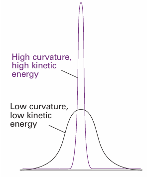
Fig. 8.26 Even if a wavefunction does not have the form of a periodic wave, it is still possible to infer from it the average kinetic energy of a particle by noting its average curvature. This illustration shows two wavefunctions: the sharply curved function corresponds to a higher kinetic energy than the less sharply curved function.
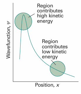
Fig. 8.27The observed kinetic energy of a particle is an average of contributions from the entire space covered by the wavefunction. Sharply curved regions contribute a high kinetic energy to the average; slightly curved regions contribute only a small kinetic energy.
 الاكثر قراءة في مواضيع عامة في الكيمياء الفيزيائية
 اخر الاخبار
اخبار العتبة العباسية المقدسة


