The perfect gas law
We assume that the following individual gas laws are familiar: Boyle’s law: pV=constant, at constant n, T (1.5) ° Charles’s law: V=constant×T, at constant n, p (1.6a) ° , p=constant×T, at constant n, V (1.6b) ° Avogadro’s principle:2V=constant×nat constant p, T (1.7)° Boyle’s and Charles’s laws are examples of a limiting law, a law that is strictly true only in a certain limit, in this case p→0. Equations valid in this limiting sense will be signalled by a °on the equation number, as in these expressions. Avogadro’s principle is commonly expressed in the form ‘equal volumes of gases at the same temperature and pressure contain the same numbers of molecules’. In this form, it is increasingly true as p→0. Although these relations are strictly true only at p=0, they are reasonably reliable at normal pressures (p≈1 bar) and are used widely throughout chemistry.
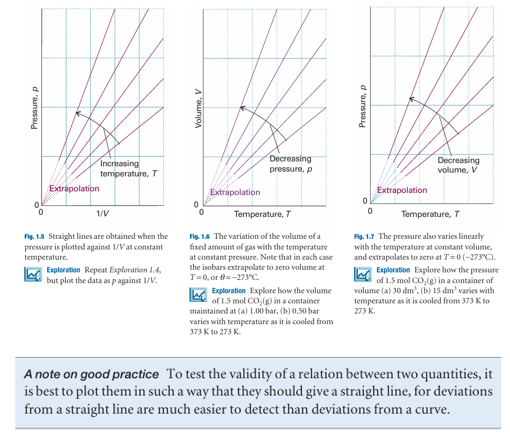
Figure 1.4 depicts the variation of the pressure of a sample of gas as the volume is changed. Each of the curves in the graph corresponds to a single temperature and hence is called an isotherm. According to Boyle’s law, the isotherms of gases are hyperbolas. An alternative depiction, a plot of pressure against 1/volume, is shown in Fig. 1.5. The linear variation of volume with temperature summarized by Charles’s law is illustrated in Fig. 1.6. The lines in this illustration are examples of isobars, or lines showing the variation of properties at constant pressure. Figure 1.7 illustrates the linear variation of pressure with temperature. The lines in this diagram are isochores, or lines showing the variation of properties at constant volume
2 Avogadro’s principle is a principle rather than a law (a summary of experience) because it depends on the validity of a model, in this case the existence of molecules. Despite there now being no doubt about the existence of molecules, it is still a model-based principle rather than a law. 3 To solve this and other Explorations, use either mathematical software or the Living graphs from the text’s web site.
The empirical observations summarized by eqns 1.5–7 can be combined into a single expression:
pV=constant ×nT
This expression is consistent with Boyle’s law (pV = constant) when n and T are constant, with both forms of Charles’s law (p ∝ T, V ∝ T) when n and either V or p are held constant, and with Avogadro’s principle (V ∝ n) when p and T are constant. The constant of proportionality, which is found experimentally to be the same for all gases, is denoted R and called the gas constant. The resulting expression
pV=nRT
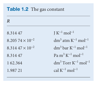
is the perfect gas equation. It is the approximate equation of state of any gas, and becomes increasingly exact as the pressure of the gas approaches zero. A gas that obeys eqn 1.8 exactly under all conditions is called a perfect gas (or ideal gas). A real gas, an actual gas, behaves more like a perfect gas the lower the pressure, and is described exactly by eqn 1.8 in the limit of p → 0. The gas constant R can be determined by evaluating R = pV/nT for a gas in the limit of zero pressure (to guarantee that it is behaving perfectly). However, a more accurate value can be obtained by measuring the speed of sound in a low-pressure gas (argon is used in practice) and extrapolating its value to zero pressure. Table 1.2 lists the values of Rin a variety of units.
Molecular interpretation 1.1 The kinetic model of gases
The molecular explanation of Boyle’s law is that, if a sample of gas is compressed to half its volume, then twice as many molecules strike the walls in a given period of time than before it was compressed. As a result, the average force exerted on the walls is doubled. Hence, when the volume is halved the pressure of the gas is doubled, and p×Vis a constant. Boyle’s law applies to all gases regardless of their chemical identity (provided the pressure is low) because at low pressures the average separation of molecules is so great that they exert no influence on one another and hence travel independently. The molecular explanation of Charles’s law lies in the fact that raising the temperature of a gas increases the average speed of its molecules. The molecules collide with the walls more frequently and with greater impact. Therefore they exert a greater pressure on the walls of the container. These qualitative concepts are expressed quantitatively in terms of the kinetic model of gases, which is described more fully in Chapter 21. Briefly, the kinetic model is based on three assumptions:
1. The gas consists of molecules of mass min ceaseless random motion.
2. The size of the molecules is negligible, in the sense that their diameters are much smaller than the average distance travelled between collisions.
3. The molecules interact only through brief, infrequent, and elastic collisions. Anelastic collision is a collision in which the total translational kinetic energy of the molecules is conserved. From the very economical assumptions of the kinetic model, it can be deduced (as we shall show in detail in Chapter 21) that the pressure and volume of the gas are related by
pV= 1/3nMc2 whereM= mNA, the molar mass of the molecules, and cis the root mean square speed of the molecules, the square root of the mean of the squares of the speeds, v, of the molecules:
c= (v2)1/2 We see that, if the root mean square speed of the molecules depends only on the temperature, then at constant temperature pV=constant which is the content of Boyle’s law. Moreover, for eqn 1.9 to be the equation of state of a perfect gas, its right-hand side must be equal to nRT. It follows that the root mean square speed of the molecules in a gas at a temperature Tmust be  We can conclude that the root mean square speed of the molecules of a gas is proportional to the square root of the temperature and inversely proportional to the square root of the molar mass. That is, the higher the temperature, the higher the root mean square speed of the molecules, and, at a given temperature, heavy molecules travel more slowly than light molecules. The root mean square speed of N2molecules, for instance, is found from eqn 1.11 to be 515 m s−1at 298K.
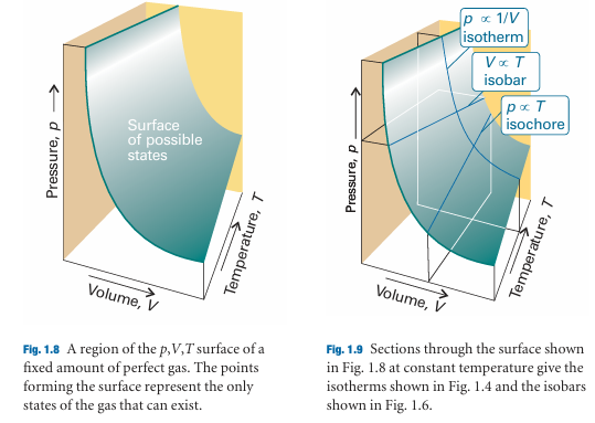
The surface in Fig. 1.8 is a plot of the pressure of a fixed amount of perfect gas against its volume and thermodynamic temperature as given by eqn 1.8. The surface depicts the only possible states of a perfect gas: the gas cannot exist in states that do not correspond to points on the surface. The graphs in Figs. 1.4 and 1.6 correspond to the sections through the surface (Fig. 1.9).
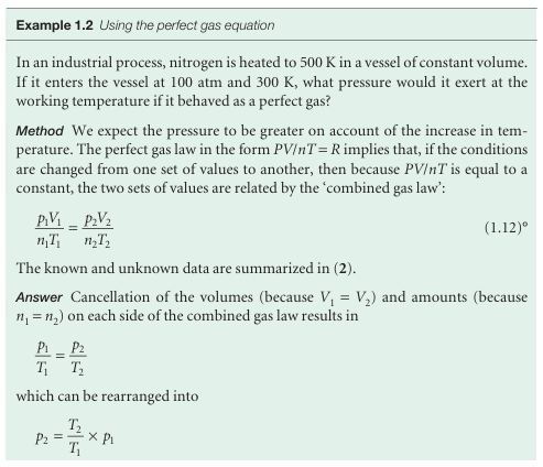
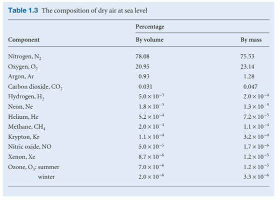
The perfect gas equation is of the greatest importance in physical chemistry because it is used to derive a wide range of relations that are used throughout thermodynamics. However, it is also of considerable practical utility for calculating the properties of a gas under a variety of conditions. For instance, the molar volume, Vm = V/n, of a perfect gas under the conditions called standard ambient temperature and pressure (SATP), which means 298.15 K and 1 bar (that is, exactly 105 Pa), is easily calculated from Vm=RT/pto be 24.789 dm3mol−1. An earlier definition, standard temperature and pressure (STP), was 0°C and 1 atm; at STP, the molar volume of a perfect gas is 22.414 dm3mol−1. Among other applications, eqn 1.8 can be used to discuss processes in the atmosphere that give rise to the weather. The biggest sample of gas readily accessible to us is the atmosphere, a mixture of gases with the composition summarized in Table 1.3. The composition is maintained moderately constant by diffusion and convection (winds, particularly the local turbulence called eddies) but the pressure and temperature vary with altitude and with the local conditions, particularly in the troposphere (the ‘sphere of change’), the layer extending up to about 11 km.
In the troposphere the average temperature is 15°C at sea level, falling to –57°C at the bottom of the tropopause at 11 km. This variation is much less pronounced when expressed on the Kelvin scale, ranging from 288 K to 216 K, an average of 268 K. If we suppose that the temperature has its average value all the way up to the tropopause, then the pressure varies with altitude, h, according to the barometric formula:
p =p0e−h/H
where p0 is the pressure at sea level and H is a constant approximately equal to 8 km. More specifically, H = RT/Mg, where M is the average molar mass of air and T is the temperature. The barometric formula fits the observed pressure distribution quite well even for regions well above the troposphere (see Fig. 1.10). It implies that the pressure of the air and its density fall to half their sea-level value at h = H ln 2, or 6 km. Local variations of pressure, temperature, and composition in the troposphere are manifest as ‘weather’. A small region of air is termed a parcel. First, we note that a parcel of warm air is less dense than the same parcel of cool air. As a parcel rises, it expands adiabatically (that is, without transfer of heat from its surroundings), so it cools. Cool air can absorb lower concentrations of water vapour than warm air, so the moisture forms clouds. Cloudy skies can therefore be associated with rising air and clear skies are often associated with descending air. The motion of air in the upper altitudes may lead to an accumulation in some regions and a loss of molecules from other regions. The former result in the formation of regions of high pressure (‘highs’ or anticyclones) and the latter result in regions of low pressure (‘lows’, depressions, or cyclones). These regions are shown as H and L on the accompanying weather map (Fig. 1.11). The lines of constant pressure—differing by 4 mbar (400 Pa, about 3 Torr)—marked on it are called isobars. The elongated regions of high and low pressure are known, respectively, as ridges and troughs. In meteorology, large-scale vertical movement is called convection. Horizontal pressure differentials result in the flow of air that we call wind (see Fig.1.12). Winds coming from the north in the Northern hemisphere and from the south in the Southern hemisphere are deflected towards the west as they migrate from a region where the Earth is rotating slowly (at the poles) to where it is rotating most rapidly (at the equator). Winds travel nearly parallel to the isobars, with low pressure to their left in the Northern hemisphere and to the right in the Southern hemisphere. At the surface, where wind speeds are lower, the winds tend to travel perpendicular to the isobars from high to low pressure. This differential motion results in a spiral outward f low of air clockwise in the Northern hemisphere around a high and an inward counter clockwise flow around a low.
The air lost from regions of high pressure is restored as an influx of air converges into the region and descends. As we have seen, descending air is associated with clear skies. It also becomes warmer by compression as it descends, so regions of high pressure are associated with high surface temperatures. In winter, the cold surface air may prevent the complete fall of air, and result in a temperature inversion, with a layer of warm air over a layer of cold air. Geographical conditions may also trap cool air, as in Los Angeles, and the photochemical pollutants we know as smog may be trapped under the warm layer.
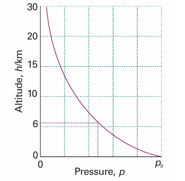
Fig. 1.10 The variation of atmospheric pressure with altitude, as predicted by the barometric formula and as suggested by the ‘US Standard Atmosphere’, which takes into account the variation of temperature with altitude.
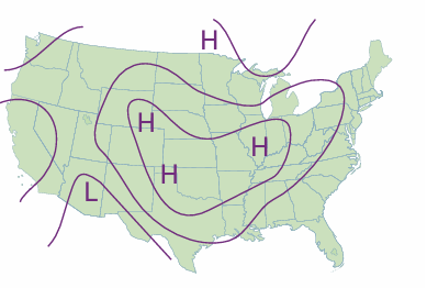
Fig. 1.11 A typical weather map; in this case, for the United States on 1 January 2000.
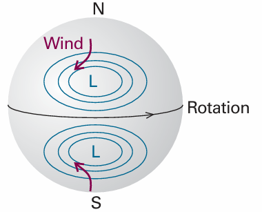
Fig. 1.12 The flow of air (‘wind’) around regions of high and low pressure in the Northern and Southern hemispheres.
 الاكثر قراءة في مواضيع عامة في الكيمياء الفيزيائية
 اخر الاخبار
اخبار العتبة العباسية المقدسة


